Mataveid V7.0

Mataveid is a basic system identification toolbox for both GNU Octave and MATLAB®. Mataveid is based on the power of linear algebra and the library is easy to use. Mataveid using the classical realization and polynomal theories to identify state space models from data. There are lots of subspace methods in the "old" folder and the reason why I'm not using these files is because they can't handle noise quite well.

I'm building this library because I feel that the commercial libraries are just for theoretical experiments. I'm focusing on real practice and solving real world problems.

UPDATE

I will update this repository with new algorithms and sorting out some of algorithms that I find is obeselete in current indistrual use.
I'm planning to add a square root unscented kalman filter and a neural network trainer with unscented kalman filter.

Caution

Installing GNU Octave's Control-Toolbox or MATLAB's Control-Toolbox/System Identification Toolbox WILL cause problems with MataveID & MataveControl because they are using the same function names.

Functions and its purpose

• OKID for multivariable hydraulic systems or temperature systems
• ERA-DC for mechanical damped systems in the time plane
• SINDY for multivariable abritary nonlinear systems
• RLS for all kind of arbitary single input and single output systems (Use this first!)
• OCID for linear feedback systems (I haven't found any real world practice for this method yet)
• FILTFILT2 for low pass filtering without phase delay
• SPA for spectral analysis
• IDBODE for mechanical damped systems in the frequency plane

Papers:

Mataveid contains realization identification and polynomal algorithms. They can be quite hard to understand, so I highly recommend to read papers in the "reports" folder about the realization identification algorithms if you want to understand how they work.

Literature:

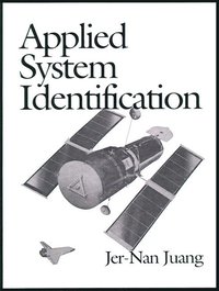
All of these methods can be found in Jer-Nan Juang's excellent and practical book Applied System Identification.
There are many good books about system identification, but if you want to make it easy, study easy and apply practical for implementation, then this book is for you.

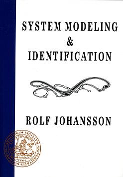
If you want to have another excellent practical book with full of applied examples, I recommending "System Modeling and Identification" by Rolf Johansson. This book coveres Recursive Least Square algorithm best.

Can be purchased from https://kfsab.se/sortiment/system-modeling-and-identification/

OKID – Observer Kalman Filter Identification

OKID is an algoritm that creates the impulse makrov parameter response from data for identify a state space model and also a kalman filter gain matrix. Use this if you got regular data from a dynamical system. This algorithm can handle both SISO and MISO. OKID have it's orgin from Hubble Telescope at NASA. This algorithm was invented 1991. The drawback with OKID algorithm is that it's very extremely sensitive to noise. So I have modify OKID by including SINDy algorithm and Euler simulation plus Algebraic Riccati Equations for finding the discrete kalman gain matrix K. So now it's very robust against noise.

[sysd, K] = okid(inputs, states, derivatives, t, sampleTime);

Example OKID

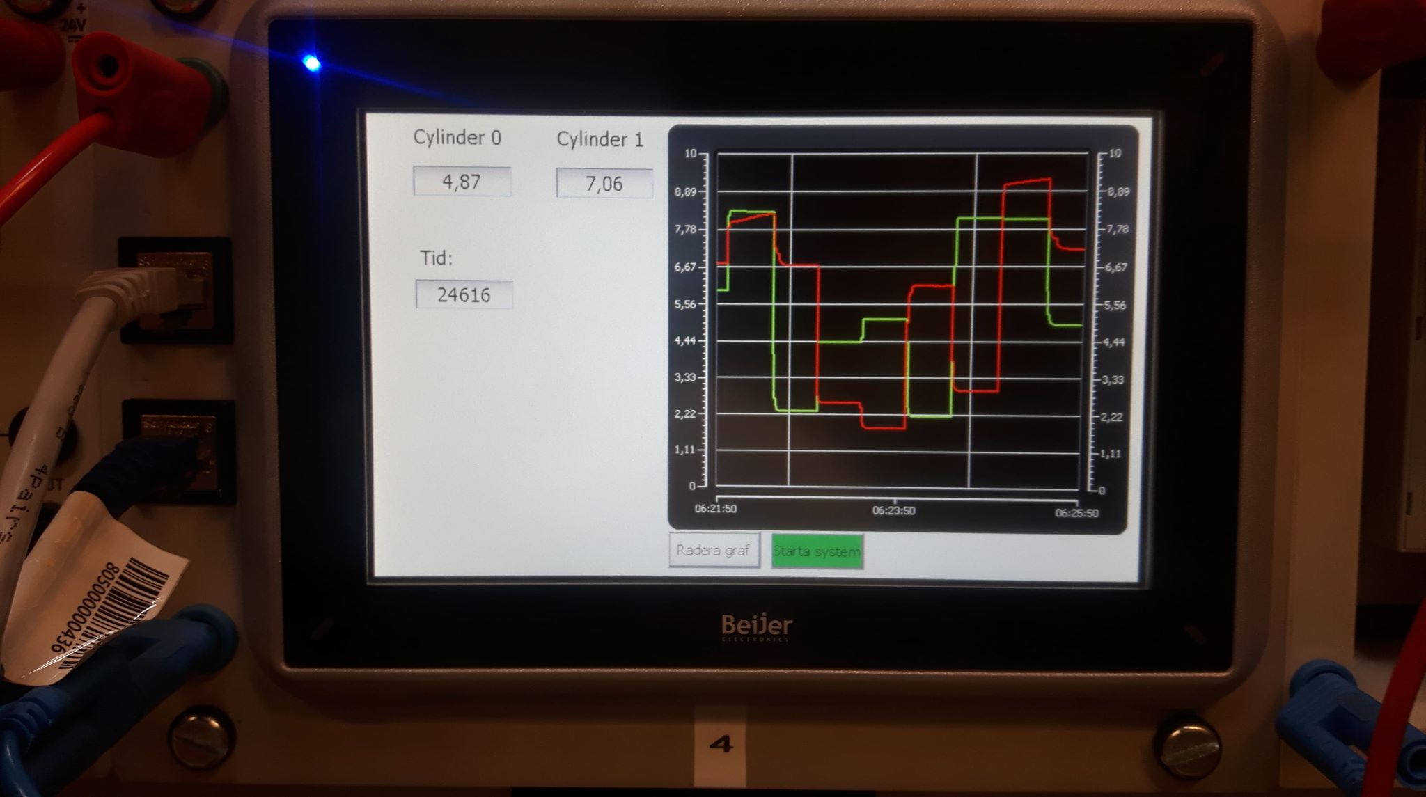
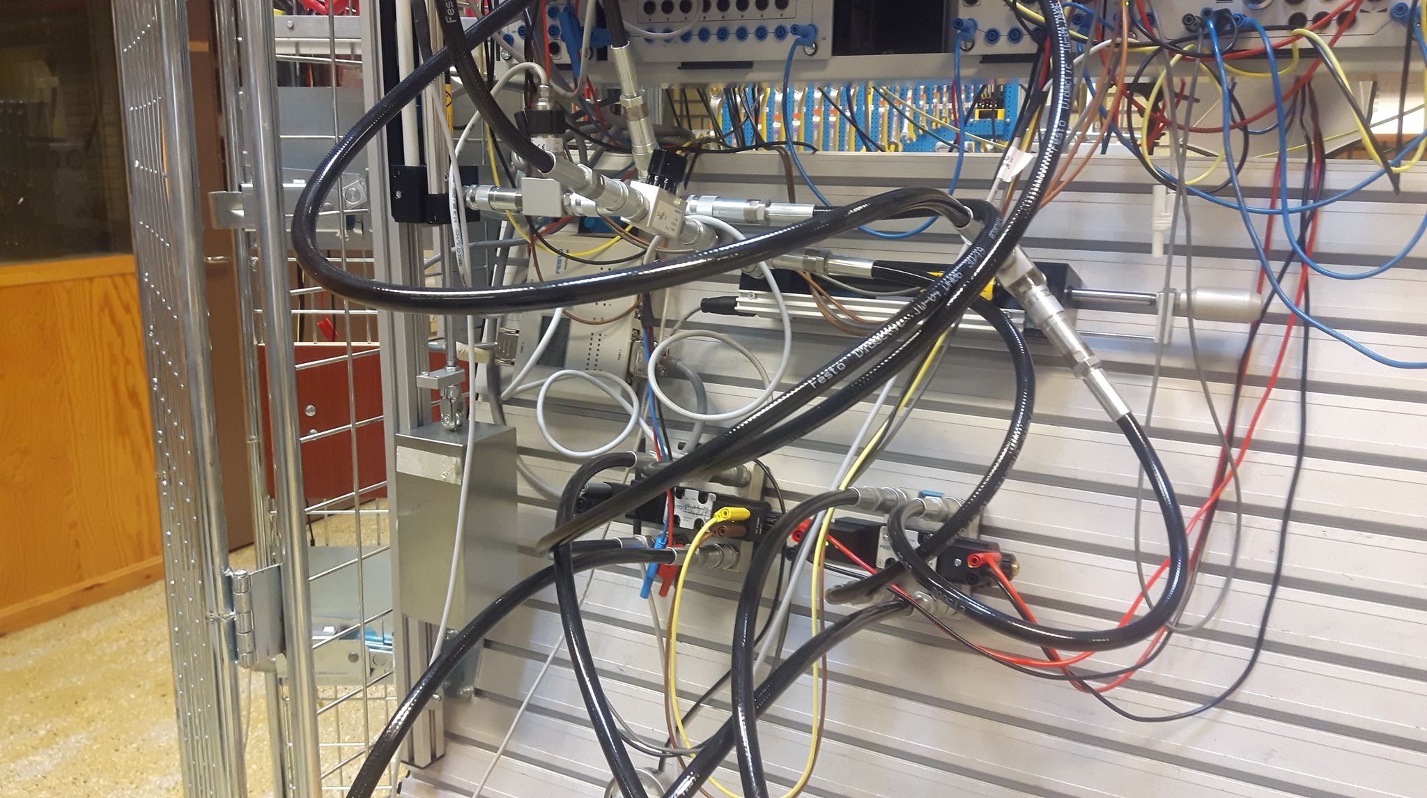
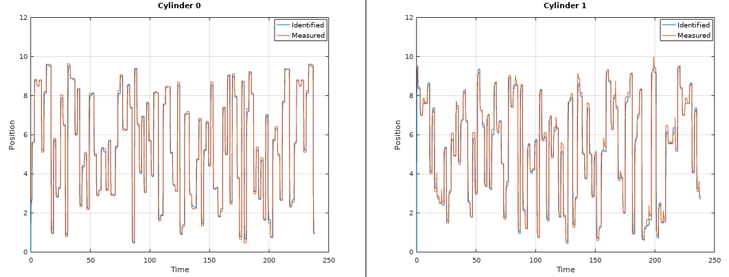
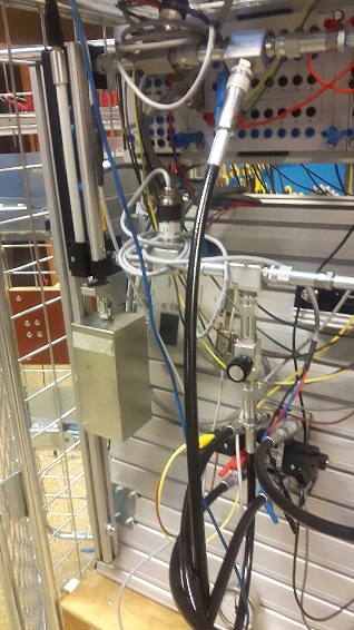
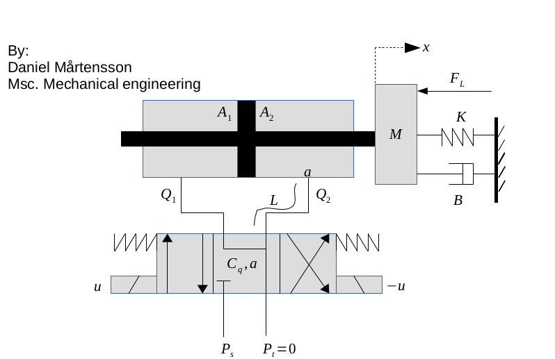
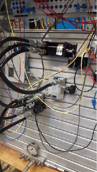
Here I programmed a Beijer PLC that controls the multivariable cylinder system. It's a nonlinear system, but OKID can handle it because it's not so nonlinear as a hydraulic motor. Cylinder 0 and Cylinder 1 affecting each other when the propotional control valves opens.

% Load the data
X = csvread('MultivariableCylinders.csv');
t = X(:, 1);
r0 = X(:, 2);
r1 = X(:, 3);
y0 = X(:, 4);
y1 = X(:, 5);
sampleTime = 0.1;

% Create the model
inputs = [r0';r1'];
states = [y0';y1'];
derivatives = (states(:, 2:end) - states(:, 1:end-1))/sampleTime;
states = states(:, 1:end-1);
inputs = inputs(:, 1:end-1);
t = t'(1, 1:end-1);
[sysd, K] = okid(inputs, states, derivatives', t, sampleTime);

% Do simulation
[outputs, T, x] = lsim(sysd ,inputs, t);
close
plot(T, outputs(1, :), t, states(1, :))
title('Cylinder 0');
xlabel('Time');
ylabel('Position');
grid on
legend('Identified', 'Measured');
ylim([0 12]);
figure
plot(T, outputs(2, :), t, states(2, :))
title('Cylinder 1');
xlabel('Time');
ylabel('Position');
grid on
legend('Identified', 'Measured');
ylim([0 12]);

RLS – Recursive Least Squares

RLS is an algorithm that creates a transfer function model from regular data. Here you can select if you want to estimate an ARX model or an ARMAX model, depending on the number of zeros in the polynomal "nze". Select number of error-zeros-polynomal "nze" to 1, and you will get a ARX model or select "nze" equal to model poles "np", you will get an ARMAX model that also includes a kalman gain matrix K. I recommending that. This algorithm can handle data with high noise, but you will only get a SISO model from it. This algorithm was invented 1821 by Gauss, but it was until 1950 when it got its attention in adaptive control.

Use this algorithm if you have regular data from a open loop system and you want to apply that algorithm into embedded system that have low RAM and low flash memory. RLS is very suitable for system that have a lack of memory.

There is a equivalent C-code for RLS algorithm here. Works on ALL embedded systems.
https://github.com/DanielMartensson/CControl

[sysd, K] = rls(u, y, np, nz, nze, sampleTime, forgetting);

Example RLS

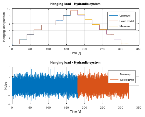
This is a hanging load of a hydraulic system. This system is a linear system due to the hydraulic cylinder that lift the load. Here I create two linear first order models. One for up lifting up and one for lowering down the weight. I'm also but a small orifice between the outlet and inlet of the hydraulic cylinder. That's create a more smooth behavior. Notice that this RLS algorithm also computes a Kalman gain matrix.

% Load data
X = csvread('HangingLoad.csv');
t = X(:, 1); % Time
r = X(:, 2); % Reference 
y = X(:, 3); % Output position
u = X(:, 4); % Input signal from P-controller with gain 3
sampleTime = 0.02;
 
% Do identification of the first data set
l = length(r) + 2000; % This is half data

% Do identification on up and down
sysd_up = rls(r(1:l/2), y(1:l/2), 1, 1, 1, sampleTime);
sysd_down = rls(r(l/2+1:end), y(l/2+1:end), 1, 1, 1, sampleTime);

% Simulate 
[~,~,x] = lsim(sysd_up, r'(1:l/2), t'(1:l/2));
hold on
lsim(sysd_down, r'(l/2+1:end), t'(l/2+1:end), x(:, end));
hold on
plot(t, y);
legend('Up model', 'Down model', 'Measured');
title('Hanging load - Hydraulic system')
xlabel('Time [s]')
ylabel('Position');

Here we can se that the first model follows the measured position perfect. The "down-curve" should be measured a little bit longer to get a perfect linear model.

ERA/DC – Eigensystem Realization Algorithm Data Correlations

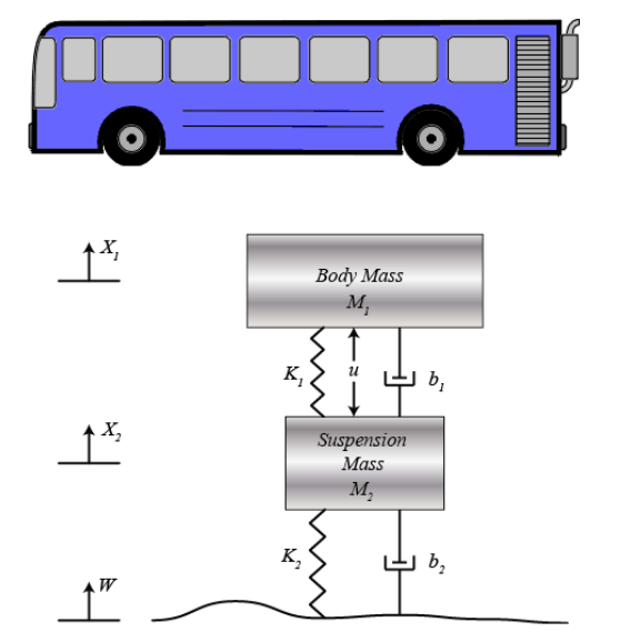
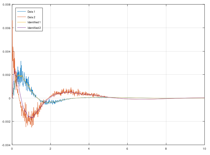
ERA/DC was invented 1987 and is a successor from ERA, that was invented 1985 at NASA. The difference between ERA/DC and ERA is that ERA/DC can handle noise much better than ERA. But both algorihtm works as the same. ERA/DC want an impulse response. e.g called markov parameters. You will get a state space model from this algorithm. This algorithm can handle both SISO and MISO data.

Use this algorithm if you got impulse data from e.g structural mechanics.

[sysd] = eradc(g, sampleTime, systemorder);

Example ERA/DC

%% Parameters
m1 = 2.3;
m2 = 3.1;
k1 = 8.5;
k2 = 5.1;
b1 = 3.3;
b2 = 5.1;

A=[0                 1   0                                              0
  -(b1*b2)/(m1*m2)   0   ((b1/m1)*((b1/m1)+(b1/m2)+(b2/m2)))-(k1/m1)   -(b1/m1)
   b2/m2             0  -((b1/m1)+(b1/m2)+(b2/m2))                      1
   k2/m2             0  -((k1/m1)+(k1/m2)+(k2/m2))                      0];
B=[0;                 
   1/m1;              
   0;                
   (1/m1)+(1/m2)];
C=[0 0 1 0];
D=[0];
delay = 0;

%% Model
buss = ss(delay,A,B,C,D);

%% Simulation
[g, t] = impulse(buss, 10);

%% Add 15% noise
load v
for i = 1:length(g)-1
  noiseSigma = 0.15*g(i);
  noise = noiseSigma*v(i); % v = noise, 1000 samples -1 to 1
  g(i) = g(i) + noise;
end

%% Identification  
systemorder = 4;
[sysd] = eradc(g, t(2) - t(1), systemorder);
    
%% Validation
gt = impulse(sysd, 10);
close
    
%% Check
plot(t, g, t, gt(:, 1:2:end))
legend("Data", "Identified", 'location', 'northwest')
grid on

OCID – Observer Controller Identification

This is an extention from OKID. The idea is the same, but OCID creates a LQR contol law as well. This algorithm works only for closed loop data. It have its orgin from NASA around 1992 when NASA wanted to identify a observer, model and a LQR control law from closed loop data that comes from an actively controlled aircraft wing in a wind tunnel at NASA Langley Research Center. This algorithm works for both SISO and MIMO models.

Use this algorithm if you want to extract a LQR control law, kalman observer and model from a running dynamical system. Or if your open loop system is unstable and it requries some kind of feedback to stabilize it. Then OCID is the perfect choice.

[sysd, K, L] = ocid(r, uf, y, sampleTime, regularization, systemorder);

OCID Example

%% Matrix A
A = [0 1  0  0; 
    -7 -5 0  1; 
     0 0  0  1;
     0 1 -8 -5];
  
%% Matrix B
B = [0 0; 
     1 0; 
     0 0; 
     0 1];
  
%% Matrix C
C = [1 0 0 0; 
     0 0 0 1];
  
%% Model and signals
delay = 0;
sys = ss(delay, A, B, C);
t = linspace(0, 20, 1000);
r = [linspace(5, -11, 100) linspace(7, 3, 100) linspace(-6, 9, 100) linspace(-7, 1, 100) linspace(2, 0, 100) linspace(6, -9, 100) linspace(4, 1, 100) linspace(0, 0, 100) linspace(10, 17, 100) linspace(-30, 0, 100)];
r = [r;2*r]; % MIMO
  
%% Feedback
Q = sys.C'*sys.C;
R = [1 4; 1 5];
L = lqr(sys, Q, R);
[feedbacksys] = reg(sys, L);
yf = lsim(feedbacksys, r, t);

%% Add 10% noise
load v
for i = 1:length(yf)
  noiseSigma = 0.10*yf(:, i);
  noise = noiseSigma*v(i); % v = noise, 1000 samples -1 to 1
  yf(:, i) = yf(:, i) + noise;
end

%% Identification  
uf = yf(3:4, :); % Input feedback signals
y = yf(1:2, :); % Output feedback signals
regularization = 600;
modelorder = 4;
[sysd, K, L] = ocid(r, uf, y, t(2) - t(1), regularization, modelorder);
    
%% Validation
u = -uf + r; % Input signal %u = -Lx + r = -uf + r
yt = lsim(sysd, u, t);
close
    
%% Check
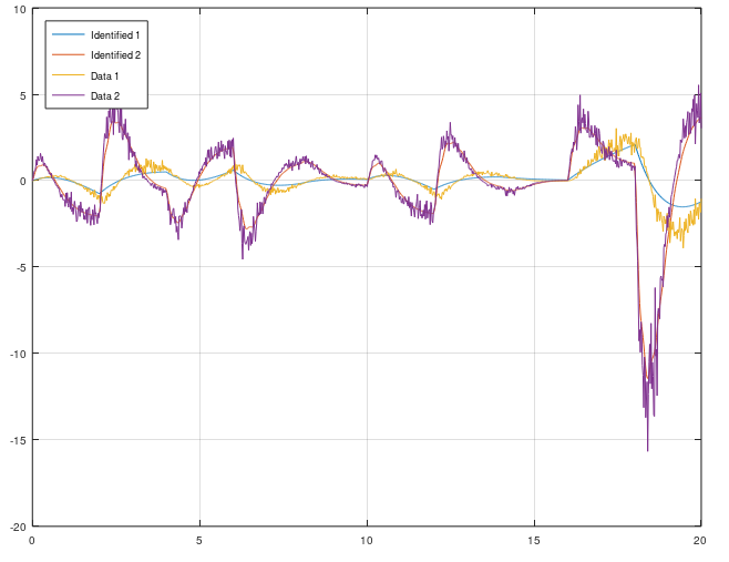
plot(t, yt(1:2, 1:2:end), t, yf(1:2, :))
legend("Identified 1", "Identified 2", "Data 1", "Data 2", 'location', 'northwest')
grid on

SINDy – Sparse Identification of Nonlinear Dynamics

This is a new identification technique made by from University of Washington. It extends the identification methods of grey-box modeling to a much simplier way. This is a very easy to use method, but still powerful because it use least squares with sequentially thresholded least squares procedure. I have made it much simpler because now it also creates the formula for the system. In more practical words, this method identify a nonlinear ordinary differential equations from time domain data.

This is very usefull if you have heavy nonlinear systems such as a hydraulic orifice or a hanging load.

SINDy Example

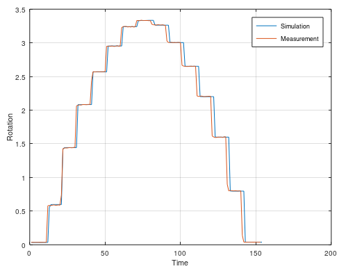
This example is a real world example with noise and nonlinearities. Here I set up a hydraulic motor in a test bench and measure it's output and the current to the valve that gives the motor oil. The motor have two nonlinearities – Hysteresis and the input signal is not propotional to the output signal. By using two nonlinear models, we can avoid the hysteresis.

% Load CSV data
X = csvread('MotorRotation.csv'); % Can be found in the folder "data"
t = X(:, 1);
u = X(:, 2);
y = X(:, 3);
sampleTime = 0.02;

% Do filtering of y
yf = filtfilt2(y', t', 0.1);

% Find the derivative of y
dy = (yf(2:end)-yf(1:end-1))/sampleTime;

% Threshold for removing noise of the derivative
for i = 1:length(dy)
  v = dy(i);
  if(and(v >= -0.15, v <= 0.15))
    dy(i) = 0;
  end
end

% Same length as dy
y = yf(1:end-1);
u = u(1:end-1);
t = t(1:end-1);

% Sindy - Sparce identification Dynamics
inputs = [u'];
states = [y];
derivatives = [dy'];
activations = [1  1  1  1  1  1  1  1  1  1  1  1  1  1  1  1  0  0  0  0  0  1  1  0  0  0  0]; % Enable or disable the candidate functions such as sin(u), x^2, sqrt(y) etc...
variables = ["y"; "u"]; % [states; inputs] - Always!
lambda = 0.1;
l = length(inputs);
h = floor(l/2);
s = ceil(l/2);
fx_up = sindy(inputs(1:h), states(1:h), derivatives(1:h), activations, variables, lambda); % We go up
fx_down = sindy(inputs(s:end), states(s:end), derivatives(s:end), activations, variables, lambda); % We go down

% Euler simulation of Sindy model by two anonymous functions
output = zeros(1, length(u));
x_up = 0;
x_down = 0;
for i = 1:length(u)
  x_up = x_up + sampleTime*fx_up{1}(x_up, u(i));
  x_down = x_down + sampleTime*fx_down{1}(x_down, u(i));
  if(i <= length(u)/2*0.91) % This is the half part of the dynamical system
    output(i) = x_up;
  else
    output(i) = x_down; % Here we go down
  end
end
plot(t, output, t, y)
legend('Model', 'Measured');
title('Hydraulic motor - Checking the hysteresis')
xlabel('Time [s]')
ylabel('Rotation');
grid on

Here is a multivariable example with SINDy. It use the same data as the OKID scenario.

X = csvread('MultivariableCylinders.csv');
t = X(:, 1);
r0 = X(:, 2);
r1 = X(:, 3);
y0 = X(:, 4);
y1 = X(:, 5);
sampleTime = 0.1;

inputs = [r0';r1'];
states = [y0';y1'];
derivatives = (states(:, 2:end) - states(:, 1:end-1))/sampleTime;
states = states(:, 1:end-1);
inputs = inputs(:, 1:end-1);
activations = [1  1  1  1  1  1  1  1  1  1  1  1  1  1  1  1  1  1  1  1  1  1  1  1  1  1  1  1  1  1  1  1  1  1  1  1  1  1  1  1  1  1  1  1  1  1  1  1  1  1  1  1  1  1  1  1  1  1  1  1  1  1  1  1  1  1  1  1  1  0  0  0  0  0  0  0  0];
lambda = 1.1;
variables = ["y0";"y1";"r0";"r1"]; % [states; inputs] - Always!
fx = sindy(inputs, states, derivatives', activations, variables, lambda);

% Euler simulation
output = zeros(2, length(t));
x0 = 0;
x1 = 0;
for i = 1:length(output)
  output(1, i) = x0;
  output(2, i) = x1;
  vy1 = fx{1}(x0, x1, r0(i), r1(i));
  vy2 = fx{2}(x0, x1, r0(i), r1(i));
  x0 = x0 + sampleTime*vy1;
  x1 = x1 + sampleTime*vy2;
end

close all
plot(t, output(2, :), t, y1);
grid on
figure
plot(t, output(1, :), t, y0);
grid on

IDBode – Identification Bode

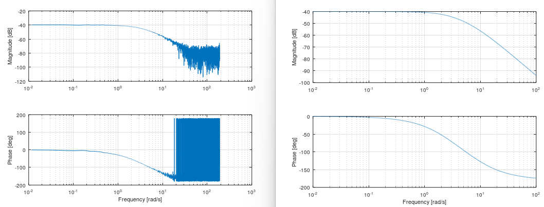
This plots a bode diagram from measurement data. It can be very interesting to see how the amplitudes between input and output behaves over frequencies. This can be used to confirm if your estimated model is good or bad by using the bode command from Matavecontrol and compare it with idebode.

idbode(u, y, w);

IDBode Example

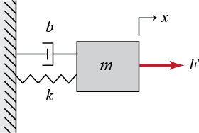
%% Model of a mass spring damper system
M = 5; % Kg
K = 100; % Nm/m
b = 52; % Nm/s^2
G = tf([1], [M b K]);

%% Frequency response
t = linspace(0.0, 50, 3000);
w = linspace(0, 100, 3000);
u = 10*sin(2*pi*w.*t);

%% Simulation
y = lsim(G, u, t);
close

%% Identify bode diagram
idbode(u, y, w);

%% Check
bode(G);

SPA – Spectral Analysis

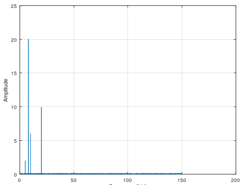
This plots all the amplitudes from noisy data over its frequencies. Very good to see what type of noise or signals you have. With this, you can determine what the real frequencies and amplitudes are and therefore you can create your filtered frequency response that are clean.

[amp, wout] = spa(y, t);

SPA Example

Assume that we are using the previous example with different parameters.

%% Model of a mass spring damper system
M = 1; % Kg
K = 500; % Nm/m
b = 3; % Nm/s^2
G = tf([1], [M b K]);

%% Frequency response
t = linspace(0.0, 100, 30000);
u1 = 10*sin(2*pi*5.*t); % 5 Hz
u2 = 10*sin(2*pi*10.*t); % 10 Hz
u3 = 10*sin(2*pi*20.*t); % 20 Hz
u4 = 10*sin(2*pi*8.*t); % 8 Hz
u = u1 + u2 + u3 + u4;

%% Simulation
y = lsim(G, u, t);
figure

%% Noise
y = y + 0.001*randn(1, 30000); 

%% Identify what frequencies we had!
spa(y, t);

Filtfilt2 – Zero Phase Filter

This filter away noise with a good old low pass filter that are being runned twice. Filtfilt2 is equal to the famous function filtfilt, but this is a regular .m file and not a C/C++ subroutine. Easy to use and recommended.

[y] = filtfilt2(y, t, K);

Filtfilt2 Example

We are using the previous example here as well.

%% Model of a mass spring damper system
M = 1; % Kg
K = 500; % Nm/m
b = 3; % Nm/s^2
G = tf([1], [M b K]);

%% Input signal
t = linspace(0.0, 100, 3000);
u = 10*sin(t);

%% Simulation
y = lsim(G, u, t);

%% Add 10% noise
load v
for i = 1:length(y)
  noiseSigma = 0.10*y(i);
  noise = noiseSigma*v(i); % v = noise, 1000 samples -1 to 1
  y(i) = y(i) + noise;
end

%% Filter away the noise
lowpass = 0.2;
[yf] = filtfilt2(y, t, lowpass);

%% Check
plot(t, yf, t, y);
legend("Filtered", "Noisy");

Install

To install Mataveid, download the folder "sourcecode" and place it where you want it. Then the following code need to be written in the terminal of your MATLAB® or GNU Octave program.

path('path/to/the/sourcecode/folder/where/all/matave/files/are/mataveid', path)
savepath

Example:

path('/home/hp/Dokument/Reglerteknik/mataveid', path)
savepath

Important! All the .m files need to be inside the folder mataveid if you want the update function to work.

Update

Write this inside the terminal. Then Mataveid is going to download new .m files to mataveid from GitHub

updatemataveid

Requirements

• Installation of Matavecontrol package https://github.com/DanielMartensson/matavecontrol